What is a mathematical model examples. Various ways to build a mathematical model

Computers have firmly entered our lives, and there is practically no such area of ​​human activity where computers would not be used. Computers are now widely used in the process of creating and researching new machines, new technological processes and looking for them best options; when deciding economic tasks, when solving the problems of planning and managing production on various levels. The creation of large objects in rocketry, aircraft construction, shipbuilding, as well as the design of dams, bridges, etc., is generally impossible without the use of computers.

To use a computer in solving applied problems, first of all, the applied problem must be "translated" into a formal mathematical language, i.e. for a real object, process or system, its mathematical model must be built.

The word "Model" comes from the Latin modus (copy, image, outline). Modeling is the replacement of some object A with another object B. The replaced object A is called the original or the modeling object, and the replacement B is called the model. In other words, a model is an object-replacement of the original object, providing the study of some properties of the original.

The purpose of modeling is to obtain, process, present and use information about objects that interact with each other and external environment; and the model here acts as a means of knowing the properties and patterns of the behavior of the object.

Mathematical modeling is a means of studying a real object, process or system by replacing them with a mathematical model that is more convenient for experimental research using a computer.

Mathematical modeling is the process of constructing and studying mathematical models of real processes and phenomena. All natural and social Sciences, using the mathematical apparatus, in fact, are engaged in mathematical modeling: they replace the real object with its model and then study the latter. As in the case of any simulation, the mathematical model does not fully describe the phenomenon under study, and questions about the applicability of the results obtained in this way are very meaningful. A mathematical model is a simplified description of reality using mathematical concepts.

A mathematical model expresses the essential features of an object or process in the language of equations and other mathematical means. Strictly speaking, mathematics itself owes its existence to what it tries to reflect, i.e. to model, in their own specific language, the patterns of the surrounding world.

At mathematical modeling the study of the object is carried out by means of a model formulated in the language of mathematics using certain mathematical methods.

The path of mathematical modeling in our time is much more comprehensive than natural modeling. A huge impetus to the development of mathematical modeling was given by the advent of computers, although the method itself was born simultaneously with mathematics thousands of years ago.

Mathematical modeling as such does not always require computer support. Each specialist professionally engaged in mathematical modeling does everything possible for the analytical study of the model. Analytical solutions (i.e., represented by formulas expressing the results of the study through the initial data) are usually more convenient and informative than numerical ones. The possibilities of analytical methods for solving complex mathematical problems, however, are very limited and, as a rule, these methods are much more complicated than numerical ones.

A mathematical model is an approximate representation of real objects, processes or systems, expressed in mathematical terms and retaining the essential features of the original. Mathematical models in a quantitative form, with the help of logical and mathematical constructions, describe the main properties of an object, process or system, its parameters, internal and external connections

All models can be divided into two classes:

1. real,
2. ideal.

In turn, real models can be divided into:

1. natural,
2. physical,
3. mathematical.

Ideal models can be divided into:

1. visual,
2. iconic,
3. mathematical.

Real full-scale models are real objects, processes and systems on which scientific, technical and industrial experiments are performed.

Real physical models are mock-ups, dummies, reproducing physical properties originals (kinematic, dynamic, hydraulic, thermal, electrical, light models).

Real mathematical are analog, structural, geometric, graphic, digital and cybernetic models.

Ideal visual models are diagrams, maps, drawings, graphs, graphs, analogues, structural and geometric models.

Ideal sign models are symbols, alphabet, programming languages, ordered notation, topological notation, network representation.

Ideal mathematical models are analytical, functional, simulation, combined models.

In the above classification, some models have a double interpretation (for example, analog). All models, except for full-scale ones, can be combined into one class of mental models, since they are the product of man's abstract thinking.

Elements of game theory

In the general case, solving the game is a rather difficult task, and the complexity of the problem and the amount of calculations required for solving increases sharply with increasing . However, these difficulties are not of a fundamental nature and are associated only with a very large volume of calculations, which in a number of cases may turn out to be practically unfeasible. The fundamental side of the method of finding a solution remains for any one and the same.

Let's illustrate this with the example of a game. Let's give it a geometric interpretation - already a spatial one. Our three strategies, we will depict with three points on the plane ; the first one lies at the origin (Fig. 1). the second and third - on the axes Oh And OU at distances 1 from the origin.

Axes I-I, II-II and III-III are drawn through the points, perpendicular to the plane . On the I-I axis, the payoffs for the strategy are plotted on the axes II-II and III-III - the payoffs for the strategies. Every enemy strategy represented by a plane that cuts off axes I-I, II-II and III-III, segments equal to winnings

with appropriate strategy and strategy . Having thus constructed all the strategies of the enemy, we will obtain a family of planes over a triangle (Fig. 2).

For this family, one can also construct a lower payoff bound, as we did in the case, and find a point N on this boundary with maximum height flat plane . This height will be the price of the game.

The frequencies of the strategies in the optimal strategy will be determined by the coordinates (x, y) points N, namely:

However, such a geometric construction, even for the case, is not easy to implement and requires a great investment of time and imagination. In the general case of the game, however, it is transferred to -dimensional space and loses all clarity, although the use of geometric terminology in some cases may be useful. When solving games in practice, it is more convenient to use not geometric analogies, but computational analytical methods, especially since these methods are the only ones suitable for solving problems on computers.

All these methods are essentially reduced to solving the problem by successive trials, but ordering the sequence of trials allows you to build an algorithm that leads to a solution in the most economical way.

Here we briefly dwell on one computational method for solving games - on the so-called "linear programming" method.

To do this, we first give a general statement of the problem of finding a solution to the game . Let the game be given T player strategies A And n player strategies IN and the payoff matrix is ​​given

It is required to find a solution to the game, i.e., two optimal mixed strategies for players A and B

where (some of the numbers and can be equal to zero).

Our optimal strategy S*A should provide us with a payoff not less than , for any behavior of the enemy, and a payoff equal to , for his optimal behavior (strategy S*B).Similarly strategy S*B must provide the enemy with a loss no greater than , for any of our behavior and equal to for our optimal behavior (strategy S*A).

The value of the game in this case is unknown to us; we will assume that it is equal to some positive number. Assuming this, we do not violate the generality of reasoning; in order to be > 0, it is obviously sufficient that all elements of the matrix be non-negative. This can always be achieved by adding a sufficiently large positive value L to the elements; in this case, the cost of the game will increase by L, and the solution will not change.

Let us choose our optimal strategy S* A . Then our average payoff for the opponent's strategy will be equal to:

Our optimal strategy S*A has the property that, for any behavior of the opponent, it provides a gain no less than ; therefore, any of the numbers cannot be less than . We get a number of conditions:

(1)

Divide inequalities (1) by a positive value and denote:

Then condition (1) can be written as

(2)

where are non-negative numbers. Because quantities satisfy the condition

We want to make our guaranteed win as high as possible; Obviously, in this case, the right side of equality (3) takes the minimum value.

Thus, the problem of finding a solution to the game is reduced to the following mathematical problem: define non-negative quantities satisfying conditions (2), so that their sum

was minimal.

Usually, when solving problems related to finding extreme values ​​(maximums and minima), the function is differentiated and the derivatives are equated to zero. But such a technique is useless in this case, since the function Ф, which need to minimize, is linear, and its derivatives with respect to all arguments are equal to one, i.e., they do not vanish anywhere. Consequently, the maximum of the function is reached somewhere on the boundary of the region of change of the arguments, which is determined by the requirement of non-negativity of the arguments and conditions (2). The method of finding extreme values ​​using differentiation is also unsuitable in those cases when the maximum of the lower (or minimum of the upper) payoff boundary is determined for the solution of the game, as we did. for example, they did it when solving games. Indeed, the lower boundary is made up of sections of straight lines, and the maximum is reached not at the point where the derivative is equal to zero (there is no such point at all), but at the boundary of the interval or at the point of intersection of straight sections.

To solve such problems, which are quite common in practice, a special apparatus has been developed in mathematics. linear programming.

The linear programming problem is posed as follows.

Given a system of linear equations:

(4)

It is required to find non-negative values ​​of quantities satisfying conditions (4) and at the same time minimizing the given homogeneous linear function of quantities (linear form):

It is easy to see that the game theory problem posed above is a particular case of the linear programming problem for

At first glance, it may seem that conditions (2) are not equivalent to conditions (4), since instead of equal signs they contain inequality signs. However, it is easy to get rid of inequality signs by introducing new fictitious non-negative variables and writing conditions (2) in the form:

(5)

The form Ф, which must be minimized, is equal to

The linear programming apparatus allows, by a relatively small number of successive samples, to select the values , satisfying the requirements. For greater clarity, here we will demonstrate the use of this apparatus directly on the material of solving specific games.

Mathematical model - this is a system of mathematical relationships - formulas, equations, inequalities, etc., reflecting the essential properties of an object or phenomenon.

Every phenomenon of nature is infinite in its complexity.. Let us illustrate this with the help of an example taken from the book by V.N. Trostnikov "Man and information" (Publishing house "Nauka", 1970).

The layman formulates the mathematics problem as follows: "How long will a stone fall from a height of 200 meters?" The mathematician will begin to create his version of the problem something like this: "We will assume that the stone is falling in the void and that the acceleration of gravity is 9.8 meters per second per second. Then..."

- Let me- can say "customer", - I don't like this simplification. I want to know exactly how long the stone will fall in real conditions, and not in a non-existent void.

- Fine, the mathematician agrees. - Let's assume that the stone has a spherical shape and a diameter... What is its approximate diameter?

- About five centimeters. But it is not spherical at all, but oblong.

- Then we will assume thathas the shape of an ellipsoid with axle shafts four, three and three centimeters and that hefalls so that the semi-major axis remains vertical all the time . We take the air pressure equal to760 mmHg , from here we find the air density...

If the one who set the problem in "human" language will not interfere further in the train of thought of a mathematician, then the latter will give a numerical answer after a while. But the "consumer" may object as before: the stone is actually not ellipsoidal at all, the air pressure in that place and at that moment was not equal to 760 mm of mercury, etc. What will the mathematician answer him?

He will answer that an exact solution of a real problem is generally impossible. Not only that stone shape, which affects air resistance, cannot be described by any mathematical equation; its rotation in flight is also beyond the control of mathematics because of its complexity. Further, the air is not uniform, since as a result of the action of random factors, fluctuations of density fluctuations arise in it. Going even deeper, one must take into account that according to the law of universal gravitation, every body acts on every other body. It follows that even the pendulum wall clock changes the trajectory of the stone with its movement.

In short, if we seriously want to accurately investigate the behavior of any object, then we first have to know the location and speed of all other objects in the universe. And this, of course. impossible .

The most effective mathematical model can be implemented on a computer in the form of an algorithmic model - the so-called "computational experiment" (see [1], paragraph 26).

Of course, the results of a computational experiment may not correspond to reality if some important aspects of reality are not taken into account in the model.

So, creating a mathematical model for solving a problem, you need to:

1. highlight the assumptions on which the mathematical model will be based;
2. determine what to consider as input data and results;
3. write down mathematical relationships that link the results with the original data.

When constructing mathematical models, it is far from always possible to find formulas that explicitly express the desired quantities through data. In such cases, mathematical methods are used to give answers of varying degrees of accuracy. There is not only mathematical modeling of any phenomenon, but also visual-natural modeling, which is provided by displaying these phenomena by means of computer graphics, i.e. the researcher is shown a kind of "computer cartoon" filmed in real time. The visibility here is very high.

Other entries

06/10/2016. 8.3. What are the main steps in the software development process? 8.4. How to control the text of the program before the output to the computer?

8.3. What are the main steps in the software development process? The process of developing a program can be expressed by the following formula: The presence of errors in a newly developed program is quite normal ...

06/10/2016. 8.5. What is debugging and testing for? 8.6. What is debugging? 8.7. What is test and testing? 8.8. What should be the test data? 8.9. What are the steps in the testing process?

8.5. What is debugging and testing for? Debugging a program is the process of finding and eliminating errors in a program based on the results of its run on a computer. Testing…

06/10/2016. 8.10. What are typical programming errors? 8.11. Does the absence of syntax errors indicate the correctness of the program? 8.12. What errors are not detected by the compiler? 8.13. What is program support?

8.10. What are typical programming errors? Mistakes can be made at all stages of solving a problem - from its formulation to execution. Varieties of errors and corresponding examples are given ...

Mathematical model b is the mathematical representation of reality.

Math modeling- the process of building and studying mathematical models.

All natural and social sciences that use the mathematical apparatus are, in fact, engaged in mathematical modeling: they replace the real object with its mathematical model and then study the latter.

Definitions.

No definition can fully cover the real-life activity of mathematical modeling. Despite this, definitions are useful in that they attempt to highlight the most significant features.

Definition of a model according to A. A. Lyapunov: Modeling is an indirect practical or theoretical study of an object, in which not the object of interest to us is directly studied, but some auxiliary artificial or natural system:

located in some objective correspondence with the cognizable object;

able to replace him in certain respects;

which, during its study, ultimately provides information about the object being modeled.

According to the textbook of Sovetov and Yakovlev: "a model is an object-substitute of the original object, which provides the study of some properties of the original." “Replacing one object with another in order to obtain information about the most important properties of the original object using the model object is called modeling.” “Under mathematical modeling we will understand the process of establishing correspondence to a given real object of some mathematical object, called a mathematical model, and the study of this model, which makes it possible to obtain the characteristics of the real object under consideration. The type of mathematical model depends on both the nature of the real object and the tasks of studying the object and the required reliability and accuracy of solving this problem.”

According to Samarsky and Mikhailov, a mathematical model is an “equivalent” of an object, reflecting in mathematical form its most important properties: the laws to which it obeys, the connections inherent in its constituent parts, etc. It exists in the triads “model-algorithm-program” . Having created the “model-algorithm-program” triad, the researcher gets a universal, flexible and inexpensive tool, which is first debugged and tested in trial computational experiments. After the adequacy of the triad to the original object is established, various and detailed “experiments” are carried out with the model, giving all the required qualitative and quantitative properties and characteristics of the object.

According to the monograph by Myshkis: “Let's move on to a general definition. Let we are going to explore some set S of properties of a real object a with

the help of mathematics. To do this, we choose a “mathematical object” a" - a system of equations, or arithmetic relations, or geometric shapes, or a combination of both, etc., the study of which by means of mathematics should answer the questions posed about the properties of S. Under these conditions, a "is called the mathematical model of the object a with respect to the totality S of its properties."

According to A. G. Sevostyanov: “A mathematical model is a set of mathematical relationships, equations, inequalities, etc., describing the main patterns inherent in the process, object or system under study.”

A somewhat less general definition of a mathematical model, based on an idealization of “input-output-state” borrowed from automata theory, is given by Wiktionary: “An abstract mathematical representation of a process, device, or theoretical idea; it uses a set of variables to represent inputs, outputs, and internal states, and sets of equations and inequalities to describe their interactions.”

Finally, the most concise definition of a mathematical model: "An equation that expresses an idea."

Formal classification of models.

The formal classification of models is based on the classification of the mathematical tools used. Often built in the form of dichotomies. For example, one of the popular sets of dichotomies is:

Linear or non-linear models; Concentrated or distributed systems; Deterministic or stochastic; Static or dynamic; discrete or continuous.

and so on. Each constructed model is linear or non-linear, deterministic or stochastic, ... Naturally, mixed types are also possible: concentrated in one respect, distributed models in another, etc.

Classification according to the way the object is represented.

Along with the formal classification, the models differ in the way they represent the object:

Structural models represent an object as a system with its own device and functioning mechanism. Functional models do not use such representations and reflect only the externally perceived behavior of the object. In their extreme expression, they are also called "black box" models. Combined types of models are also possible, which are sometimes called "grey box" models.

Almost all authors describing the process of mathematical modeling indicate that first a special ideal construction, a meaningful model, is built. There is no established terminology here, and other authors call this ideal object a conceptual model, a speculative model, or a premodel. In this case, the final mathematical construction is called a formal model or simply a mathematical model obtained as a result of the formalization of this content model. A meaningful model can be built using a set of ready-made idealizations, as in mechanics, where ideal springs, rigid bodies, ideal pendulums, elastic media, etc. provide ready-made structural elements for meaningful modeling. However, in areas of knowledge where there are no fully completed formalized theories, the creation of meaningful models becomes much more complicated.

The work of R. Peierls gives a classification of mathematical models used in physics and, more broadly, in the natural sciences. In the book by A. N. Gorban and R. G. Khlebopros, this classification is analyzed and expanded. This classification is focused primarily on the stage of constructing a meaningful model.

These models "represent a trial description of the phenomenon, and the author either believes in its possibility, or even considers it to be true." According to R. Peierls, for example, the model of the solar system according to Ptolemy and the Copernican model, Rutherford's model of the atom and the Big Bang model.

No hypothesis in science can be proven once and for all. Richard Feynman put it very clearly:

“We always have the ability to disprove a theory, but note that we can never prove that it is correct. Let's suppose that you put forward a successful hypothesis, calculate where it leads, and find that all its consequences are confirmed experimentally. Does this mean that your theory is correct? No, it simply means that you failed to refute it.

If a model of the first type is built, then this means that it is temporarily recognized as true and one can concentrate on other problems. However, this cannot be a point in research, but only a temporary pause: the status of the model of the first type can only be temporary.

The phenomenological model contains a mechanism for describing the phenomenon. However, this mechanism is not convincing enough, cannot be sufficiently confirmed by the available data, or does not agree well with the available theories and accumulated knowledge about the object. Therefore, phenomenological models have the status of temporary solutions. It is believed that the answer is still unknown and it is necessary to continue the search for "true mechanisms". Peierls refers, for example, the caloric model and the quark model of elementary particles to the second type.

The role of the model in research may change over time, it may happen that new data and theories confirm the phenomenological models and they will be upgraded to

hypothesis status. Likewise, new knowledge may gradually come into conflict with models-hypotheses of the first type, and they may be transferred to the second. Thus, the quark model is gradually moving into the category of hypotheses; atomism in physics arose as a temporary solution, but with the course of history it passed into the first type. But the ether models have gone from type 1 to type 2, and now they are outside of science.

The idea of ​​simplification is very popular when building models. But simplification is different. Peierls distinguishes three types of simplifications in modeling.

If it is possible to construct equations describing the system under study, this does not mean that they can be solved even with the help of a computer. A common technique in this case is the use of approximations. Among them are linear response models. The equations are replaced by linear ones. The standard example is Ohm's law.

If we use the ideal gas model to describe sufficiently rarefied gases, then this is a type 3 model. At higher gas densities, it is also useful to imagine a simpler ideal gas situation for qualitative understanding and evaluation, but then this is already type 4.

In a type 4 model, details are discarded that can noticeably and not always controllably affect the result. The same equations can serve as a Type 3 or Type 4 model, depending on the phenomenon the model is used to study. So, if linear response models are used in the absence of more complex models, then these are already phenomenological linear models, and they belong to the following type 4.

Examples: application of an ideal gas model to a non-ideal one, the van der Waals equation of state, most models of solid state, liquid and nuclear physics. The path from microdescription to the properties of bodies consisting of a large number of particles is very long. Many details have to be left out. This leads to models of the 4th type.

The heuristic model retains only a qualitative similarity to reality and makes predictions only "in order of magnitude". A typical example is the mean free path approximation in kinetic theory. It gives simple formulas for coefficients of viscosity, diffusion, thermal conductivity, consistent with reality in order of magnitude.

But when building a new physics, it is far from immediately obtained a model that gives at least a qualitative description of an object - a model of the fifth type. In this case, a model is often used by analogy, reflecting reality at least in some way.

R. Peierls cites the history of the use of analogies in W. Heisenberg's first article on nature nuclear forces. “This happened after the discovery of the neutron, and although W. Heisenberg himself understood that nuclei could be described as consisting of neutrons and protons, he still could not get rid of the idea that the neutron should ultimately consist of a proton and an electron. In this case, an analogy arose between the interaction in the neutron-proton system and the interaction of a hydrogen atom and a proton. It was this analogy that led him to the conclusion that there must be exchange forces of interaction between a neutron and a proton, which are analogous to the exchange forces in the H − H system, due to the transition of an electron between two protons. ... Later, the existence of exchange forces of interaction between a neutron and a proton was nevertheless proved, although they were not completely exhausted

interaction between two particles ... But, following the same analogy, W. Heisenberg came to the conclusion that there are no nuclear forces of interaction between two protons and to the postulation of repulsion between two neutrons. Both of these latter findings are in conflict with the findings of later studies.

A. Einstein was one of the great masters of the thought experiment. Here is one of his experiments. It was conceived in youth and eventually led to the construction special theory relativity. Suppose that in classical physics we follow a light wave at the speed of light. We will observe an electromagnetic field periodically changing in space and constant in time. According to Maxwell's equations, this cannot be. From this, young Einstein concluded: either the laws of nature change when the frame of reference changes, or the speed of light does not depend on the frame of reference. He chose the second - more beautiful option. Another famous Einstein thought experiment is the Einstein-Podolsky-Rosen Paradox.

And here is type 8, which is widely used in mathematical models of biological systems.

These are also thought experiments with imaginary entities, demonstrating that the alleged phenomenon is consistent with the basic principles and is internally consistent. This is the main difference from models of type 7, which reveal hidden contradictions.

One of the most famous such experiments is Lobachevsky's geometry. Another example is the mass production of formally kinetic models of chemical and biological oscillations, autowaves, etc. The Einstein-Podolsky-Rosen paradox was conceived as a type 7 model to demonstrate inconsistency quantum mechanics. In a completely unplanned way, it eventually turned into a type 8 model - a demonstration of the possibility of quantum teleportation of information.

Consider mechanical system, consisting of a spring fixed at one end and a load of mass m attached to the free end of the spring. We will assume that the load can only move in the direction of the spring axis. Let us construct a mathematical model of this system. We will describe the state of the system by the distance x from the center of the load to its equilibrium position. We describe the interaction of a spring and a load using Hooke's law, after which we use Newton's second law to express it in the form of a differential equation:

where means the second derivative of x with respect to time..

The resulting equation describes the mathematical model of the considered physical system. This pattern is called the "harmonic oscillator".

According to the formal classification, this model is linear, deterministic, dynamic, concentrated, continuous. In the process of building it, we made many assumptions that may not be true in reality.

In relation to reality, this is, most often, a type 4 model, a simplification, since some essential universal features are omitted. In some approximation, such a model describes a real mechanical system quite well, since

discarded factors have a negligible influence on its behavior. However, the model can be refined by taking into account some of these factors. This will lead to a new model, with a wider scope.

However, when the model is refined, the complexity of its mathematical study can increase significantly and make the model virtually useless. Often, a simpler model allows you to better and deeper explore the real system than a more complex one.

If we apply the harmonic oscillator model to objects that are far from physics, its meaningful status may be different. For example, when applying this model to biological populations, it should most likely be attributed to type 6 analogy.

Hard and soft models.

The harmonic oscillator is an example of a so-called "hard" model. It is obtained as a result of a strong idealization of a real physical system. To resolve the issue of its applicability, it is necessary to understand how significant are the factors that we have neglected. In other words, it is necessary to investigate the "soft" model, which is obtained by a small perturbation of the "hard" one. It can be given, for example, by the following equation:

Here - some function, which can take into account the friction force or the dependence of the coefficient of stiffness of the spring on the degree of its stretching, ε - some small parameter. The explicit form of the function f does not interest us at the moment. If we prove that the behavior of a soft model is not fundamentally different from the behavior of a hard model, the problem will be reduced to the study of a hard model. Otherwise, the application of the results obtained in the study of the rigid model will require additional research. For example, the solution to the equation of a harmonic oscillator are functions of the form

That is, oscillations with a constant amplitude. Does it follow from this that a real oscillator will oscillate indefinitely with a constant amplitude? No, because considering a system with an arbitrarily small friction, we get damped oscillations. The behavior of the system has changed qualitatively.

If a system retains its qualitative behavior under a small perturbation, it is said to be structurally stable. The harmonic oscillator is an example of a structurally unstable system. However, this model can be used to study processes over limited time intervals.

Model versatility.

The most important mathematical models usually have an important property of universality: fundamentally different real phenomena can be described by the same mathematical model. For example, a harmonic oscillator describes not only the behavior of a load on a spring, but also other oscillatory processes, often of a completely different nature: small oscillations of a pendulum, fluctuations in the liquid level in a U-shaped vessel, or a change in the current strength in an oscillatory circuit. Thus, studying one mathematical model, we study at once a whole class of phenomena described by it. It is this isomorphism of laws expressed by mathematical models in various segments scientific knowledge, the feat of Ludwig von Bertalanffy to create " general theory systems."

Direct and inverse problems of mathematical modeling

There are many problems associated with mathematical modeling. First, it is necessary to come up with the basic scheme of the object being modeled, to reproduce it within the framework of the idealizations of this science. So, the train car turns into a system of plates and more complex

bodies from different materials, each material is specified as its standard mechanical idealization, after which equations are compiled, along the way some details are discarded as insignificant, calculations are made, compared with measurements, the model is refined, and so on. However, for the development of mathematical modeling technologies, it is useful to disassemble this process into its main constituent elements.

Traditionally, there are two main classes of problems associated with mathematical models: direct and inverse.

Direct task: the structure of the model and all its parameters are considered known, the main task is to study the model in order to extract useful knowledge about the object. What static load can the bridge withstand? How it will react to a dynamic load, how the plane will overcome the sound barrier, whether it will fall apart from flutter - these are typical examples of a direct problem. The formulation of a correct direct problem requires special skill. If the right questions are not asked, the bridge may collapse even if it was built. good model for his behaviour. So, in 1879 in the UK, a metal bridge across the River Tey collapsed, the designers of which built a model of the bridge, calculated it for a 20-fold safety margin for the payload, but forgot about the winds constantly blowing in those places. And after a year and a half it collapsed.

IN In the simplest case, the direct problem is very simple and reduces to an explicit solution of this equation.

Inverse problem: a set of possible models is known, it is necessary to choose a specific model based on additional data about the object. Most often, the structure of the model is known and some unknown parameters need to be determined. Additional information may consist in additional empirical data, or in the requirements for the object. Additional data can come independently of the process of solving the inverse problem or be the result of an experiment specially planned in the course of solving.

One of the first examples of a virtuoso solution of an inverse problem with the fullest possible use of available data was the method constructed by I. Newton for reconstructing friction forces from observed damped oscillations.

IN Another example is mathematical statistics. The task of this science is the development of methods for recording, describing and analyzing observational and experimental data in order to build probabilistic models of mass random phenomena. Those. the set of possible models is limited by probabilistic models. In specific problems, the set of models is more limited.

Computer systems of modeling.

To support mathematical modeling, computer mathematics systems have been developed, for example, Maple, Mathematica, Mathcad, MATLAB, VisSim, etc. They allow you to create formal and block models of both simple and complex processes and devices and easily change model parameters during simulation. Block models are represented by blocks, the set and connection of which are specified by the model diagram.

Additional examples.

The growth rate is proportional to the current population size. It is described by the differential equation

where α is some parameter determined by the difference between fertility and mortality. The solution to this equation is the exponential function x = x0 e. If the birth rate exceeds the death rate, the size of the population increases indefinitely and very rapidly. It is clear that in reality this cannot happen due to the limited

resources. When a certain critical population size is reached, the model ceases to be adequate, since it does not take into account the limited resources. A refinement of the Malthus model can be the logistic model, which is described by the Verhulst differential equation

where xs is the "equilibrium" population size, at which the birth rate is exactly compensated by the death rate. The population size in such a model tends to the equilibrium value xs , and this behavior is structurally stable.

Let us suppose that two kinds of animals live in a certain territory: rabbits and foxes. Let the number of rabbits be x, the number of foxes y. Using the Malthus model with the necessary corrections, taking into account the eating of rabbits by foxes, we arrive at the following system, which bears the name of the Lotka-Volterra model:

This system has an equilibrium state when the number of rabbits and foxes is constant. Deviation from this state leads to fluctuations in the number of rabbits and foxes, similar to fluctuations in the harmonic oscillator. As in the case of a harmonic oscillator, this behavior is not structurally stable: a small change in the model can lead to a qualitative change in behavior. For example, the equilibrium state can become stable, and population fluctuations will fade. The opposite situation is also possible, when any small deviation from the equilibrium position will lead to catastrophic consequences, up to total extinction one of the types. To the question of which of these scenarios is realized, the Volterra-Lotka model does not give an answer: additional research is required here.

In the article brought to your attention, we offer examples of mathematical models. In addition, we will pay attention to the stages of creating models and analyze some of the problems associated with mathematical modeling.

Another issue of ours is mathematical models in economics, examples of which we will consider a definition a little later. We propose to start our conversation with the very concept of “model”, briefly consider their classification and move on to our main questions.

The concept of "model"

We often hear the word "model". What is it? This term has many definitions, here are just three of them:

• a specific object that is created to receive and store information, reflecting some properties or characteristics, and so on, of the original of this object (this specific object can be expressed in different form: mental, description using signs, and so on);
• a model also means a display of any specific situation, life or management;
• a small copy of an object can serve as a model (they are created for a more detailed study and analysis, since the model reflects the structure and relationships).

Based on everything that was said earlier, we can draw a small conclusion: the model allows you to study in detail a complex system or object.

All models can be classified according to a number of criteria:

• by area of ​​use (educational, experimental, scientific and technical, gaming, simulation);
• by dynamics (static and dynamic);
• by branch of knowledge (physical, chemical, geographical, historical, sociological, economic, mathematical);
• according to the method of presentation (material and informational).

Information models, in turn, are divided into sign and verbal. And iconic - on computer and non-computer. Now let's move on to a detailed consideration of examples of a mathematical model.

Mathematical model

As you might guess, a mathematical model reflects some features of an object or phenomenon using special mathematical symbols. Mathematics is needed in order to model the laws of the world in its own specific language.

The method of mathematical modeling originated quite a long time ago, thousands of years ago, along with the advent of this science. However, the impetus for the development of this modeling method was given by the appearance of computers (electronic computers).

Now let's move on to classification. It can also be carried out according to some signs. They are presented in the table below.

We invite you to stop and take a closer look. latest classification, since it reflects the general patterns of modeling and the goals of the models being created.

Descriptive Models

In this chapter, we propose to dwell in more detail on descriptive mathematical models. In order to make everything very clear, an example will be given.

To begin with, this view can be called descriptive. This is due to the fact that we simply make calculations and forecasts, but we cannot influence the outcome of the event in any way.

A striking example of a descriptive mathematical model is the calculation of the flight path, speed, distance from the Earth of a comet that invaded the expanses of our solar system. This model is descriptive, since all the results obtained can only warn us of some kind of danger. Unfortunately, we cannot influence the outcome of the event. However, based on the calculations obtained, it is possible to take any measures to preserve life on Earth.

Optimization Models

Now we will talk a little about economic and mathematical models, examples of which can be various situations. In this case, we are talking about models that help to find the right answer in certain conditions. They must have some parameters. To make it very clear, consider an example from the agrarian part.

We have a granary, but the grain spoils very quickly. In this case, we need to choose the right temperature regime and optimize the storage process.

Thus, we can define the concept of "optimization model". In a mathematical sense, this is a system of equations (both linear and not), the solution of which helps to find the optimal solution in a particular economic situation. We have considered an example of a mathematical model (optimization), but I would like to add one more thing: this type belongs to the class of extreme problems, they help to describe the functioning of the economic system.

We note one more nuance: models can be of a different nature (see the table below).

Multicriteria models

Now we invite you to talk a little about the mathematical model of multiobjective optimization. Before that, we gave an example of a mathematical model for optimizing a process according to any one criterion, but what if there are a lot of them?

A striking example of a multicriteria task is the organization of proper, healthy and at the same time economical nutrition. large groups of people. Such tasks are often encountered in the army, school canteens, summer camps, hospitals and so on.

What criteria are given to us in this task?

1. Food should be healthy.
2. Food expenses should be kept to a minimum.

As you can see, these goals do not coincide at all. This means that when solving a problem, it is necessary to look for the optimal solution, a balance between the two criteria.

Game models

Speaking about game models, it is necessary to understand the concept of "game theory". Simply put, these models reflect mathematical models of real conflicts. It is only worth understanding that, unlike a real conflict, a game mathematical model has its own specific rules.

Now I will give a minimum of information from game theory, which will help you understand what a game model is. And so, in the model there are necessarily parties (two or more), which are usually called players.

All models have certain characteristics.

The game model can be paired or multiple. If we have two subjects, then the conflict is paired, if more - multiple. An antagonistic game can also be distinguished, it is also called a zero-sum game. This is a model in which the gain of one of the participants is equal to the loss of the other.

simulation models

In this section, we will focus on simulation mathematical models. Examples of tasks are:

• model of the dynamics of the number of microorganisms;
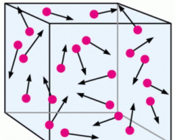
• model of molecular motion, and so on.

In this case, we are talking about models that are as close as possible to real processes. By and large, they imitate any manifestation in nature. In the first case, for example, we can model the dynamics of the number of ants in one colony. In this case, you can observe the fate of each individual. In this case, the mathematical description is rarely used, more often there are written conditions:

• after five days, the female lays eggs;
• after twenty days the ant dies, and so on.

So used to describe big system. Mathematical conclusion is the processing of the received statistical data.

Requirements

It is very important to know that there are some requirements for this type of model, among which are those given in the table below.

Modeling steps

In total, it is customary to distinguish four stages in mathematical modeling.

1. Formulation of laws linking parts of the model.
2. Study of mathematical problems.
3. Finding out the coincidence of practical and theoretical results.
4. Analysis and modernization of the model.

Economic and mathematical model

In this section, we will briefly highlight the issue. Examples of tasks can be:

• formation of a production program for the production of meat products, ensuring the maximum profit of production;
• maximizing the profit of the organization by calculating the optimal number of tables and chairs to be produced in a furniture factory, and so on.

The economic-mathematical model displays an economic abstraction, which is expressed using mathematical terms and signs.

Computer mathematical model

Examples of a computer mathematical model are:

• hydraulics tasks using flowcharts, diagrams, tables, and so on;
• problems on solid mechanics, and so on.

A computer model is an image of an object or system, presented as:

• tables;
• block diagrams;
• diagrams;
• graphics, and so on.

At the same time, this model reflects the structure and interconnections of the system.

Building an economic and mathematical model

We have already talked about what an economic-mathematical model is. An example of solving the problem will be considered right now. We need to analyze the production program to identify the reserve for increasing profits with a shift in the assortment.

We will not fully consider the problem, but only build an economic and mathematical model. The criterion of our task is profit maximization. Then the function has the form: Л=р1*х1+р2*х2… tending to the maximum. In this model, p is the profit per unit, x is the number of units produced. Further, based on the constructed model, it is necessary to make calculations and summarize.

An example of building a simple mathematical model

Task. The fisherman returned with the following catch:

• 8 fish - inhabitants of the northern seas;
• 20% of the catch - the inhabitants of the southern seas;
• not a single fish was found from the local river.

How many fish did he buy at the store?

So, an example of constructing a mathematical model of this problem is as follows. We designate total fish for x Following the condition, 0.2x is the number of fish living in southern latitudes. Now we combine all the available information and get a mathematical model of the problem: x=0.2x+8. We solve the equation and get the answer to the main question: he bought 10 fish in the store.

MATHEMATICAL MODEL - representation of a phenomenon or process studied in concrete scientific knowledge in the language of mathematical concepts. At the same time, a number of properties of the phenomenon under study are supposed to be obtained on the path of studying the actual mathematical characteristics of the model. Construction of M.m. most often dictated by the need to have a quantitative analysis of the studied phenomena and processes, without which, in turn, it is impossible to make experimentally verifiable predictions about their course.

The process of mathematical modeling, as a rule, goes through the following stages. At the first stage, the links between the main parameters of the future M.m. First of all, we are talking about a qualitative analysis of the phenomena under study and the formulation of patterns that link the main objects of research. On this basis, the identification of objects that allow a quantitative description is carried out. The stage ends with the construction of a hypothetical model, in other words, a record in the language of mathematical concepts of qualitative ideas about the relationships between the main objects of the model, which can be quantitatively characterized.

At the second stage, the study of the actual mathematical problems, to which the constructed hypothetical model leads, takes place. The main thing at this stage is to obtain empirically verifiable theoretical consequences (solution of the direct problem) as a result of the mathematical analysis of the model. At the same time, cases are not uncommon when, for the construction and study of M.m. V various fields concrete scientific knowledge, the same mathematical apparatus is used (for example, differential equations) and mathematical problems of the same type, although very non-trivial in each specific case, arise. In addition, at this stage, the use of high-speed computing technology (computer) becomes of great importance, which makes it possible to obtain an approximate solution of problems, often impossible in the framework of pure mathematics, with a previously unavailable (without the use of a computer) degree of accuracy.

The third stage is characterized by activities to identify the degree of adequacy of the constructed hypothetical M.m. those phenomena and processes for the study of which it was intended. Namely, in the event that all model parameters have been specified, the researchers try to find out how, within the accuracy of observations, their results are consistent with the theoretical consequences of the model. Deviations beyond the accuracy of observations indicate the inadequacy of the model. However, there are often cases when, when building a model, a number of its parameters remain unchanged.

indefinite. Problems in which the parametric characteristics of the model are established in such a way that the theoretical consequences are comparable within the accuracy of observations with the results of empirical tests are called inverse problems.

At the fourth stage, taking into account the identification of the degree of adequacy of the constructed hypothetical model and the emergence of new experimental data on the phenomena under study, the subsequent analysis and modification of the model takes place. Here, the decision taken varies from an unconditional rejection of the applied mathematical tools to the adoption of the constructed model as a foundation for constructing a fundamentally new scientific theory.

The first M.m. appeared in ancient science. So, to model the solar system, the Greek mathematician and astronomer Eudoxus gave each planet four spheres, the combination of the movement of which created a hippopede - a mathematical curve similar to the observed movement of the planet. Since, however, this model could not explain all the observed anomalies in the motion of the planets, it was later replaced by the epicyclic model of Apollonius from Perge. latest model used in his studies by Hipparchus, and then, subjecting it to some modification, and Ptolemy. This model, like its predecessors, was based on the belief that the planets make uniform circular motions, the overlap of which explained the apparent irregularities. At the same time, it should be noted that the Copernican model was fundamentally new only in a qualitative sense (but not as M.M.). And only Kepler, based on the observations of Tycho Brahe, built a new M.m. The solar system, proving that the planets move not in circular, but in elliptical orbits.

At present, M.m. constructed to describe mechanical and physical phenomena. On the adequacy of M.m. outside of physics one can, with a few exceptions, speak with a fair amount of caution. Nevertheless, fixing the hypotheticality, and often simply the inadequacy of M.m. in various fields of knowledge, their role in the development of science should not be underestimated. There are frequent cases when even models that are far from adequate to a large extent organized and stimulated further research, along with erroneous conclusions, contained those grains of truth that fully justified the efforts expended on developing these models.

Literature:

Math modeling. M., 1979;

Ruzavin G.I. Mathematization of scientific knowledge. M., 1984;

Tutubalin V.N., Barabasheva Yu.M., Grigoryan A.A., Devyatkova G.N., Uger E.G. Differential Equations in ecology: historical and methodological reflection // Issues of the history of natural science and technology. 1997. No. 3.

Dictionary of philosophical terms. Scientific edition of Professor V.G. Kuznetsova. M., INFRA-M, 2007, p. 310-311.